Preparing Data
Even when there is a non-linear relationship between x and y, R can estimate the parameter of a regression equation. As the data used in this page, let's generate the data that accompanied the error in accordance with the logistic growth curve. Solution of logistic growth curve are xt=K/(1+(K/x0-1)e-rt, then deform the equations as K=a, K/x0-1=b, r=c. The formula converted to y=a/(1+be-ct). In this example, we will estimate the parameters of a, b and c.
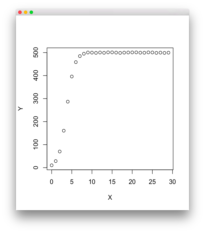
a=500; b=49; c=1.05
x <- seq(0,29,1)
y <-  a/(1+b*exp(-1*c*x)) + rnorm(30, 0, 1)
xy <- data.frame(X=x,Y=y)
plot(xy)
Non-Linear Regression Analysis by nls Function
You can perform a regression by running the commands as follows. The initial value are set, however, please try some of the initial value if it does not go well.
xy.nls <- nls(Y~a_/(1+b_*exp(-1*c_*X)),data=xy,start=list(a_=400, b_=40, c_=1.5))
summary(xy.nls)
It prints like following.
Formula: Y ~ a_/(1 + b_ * exp(-1 * c_ * X))

Parameters:
    Estimate Std. Error t value Pr(>|t|)
a_ 5.000e+02  1.873e-01 2669.16   <2e-16 ***
b_ 4.917e+01  7.898e-01   62.25   <2e-16 ***
c_ 1.048e+00  4.207e-03  249.06   <2e-16 ***
---
Signif. codes:  0 ‘***’ 0.001 ‘**’ 0.01 ‘*’ 0.05 ‘.’ 0.1 ‘ ’ 1

Residual standard error: 0.8843 on 27 degrees of freedom

Number of iterations to convergence: 7
Achieved convergence tolerance: 1.059e-06
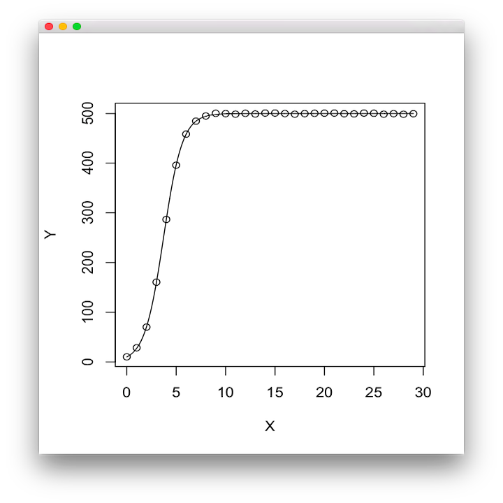
Regression result shows that a=500.0, b=49.17, c = 1.048. All coefficients are 0.1% significance. Finally, plot the approximate curve.
x2 <- seq(0, 29, length=2000)
lines(x2, predict(xy.nls, newdata=data.frame(X=x2)))